

| | 3.1 An Induction Proof |
Our first example describes the proof of the formula
sum_i=0^n i = (n+1)*n/2
using two axioms that uniquely characterize ("recursively define") the summation quantifier for every (natural number) upper bound of the summation domain:
sum_i=0^0 i = 0
sum_i=0^n i = n + sum_i=^(n-1) i (n > 0)
We start our proving session by typing the command
newcontext "sum";
(note the trailing semicolon) in the input field. This command starts a new session by erasing all previous declarations (if any) and creating a subdirectory sum of the current working directory in which the subsequently created proof will be persistently stored after the session. The system is now in "declaration mode" i.e. it accepts declarations that are entered by the user.
We now enter a constant declaration (note the trailing semicolon)
sum: NAT->NAT;
which introduces a function sum from the natural numbers to the
natural numbers (denoted by the builtin atomic type NAT).
This function will take the role of the summation quantifier:
given a number n, it shall return sum_i=0^n i. We correspondingly declare two axioms
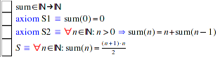
  S1: AXIOM sum(0)=0;
  S2: AXIOM FORALL(n:NAT): n>0 => sum(n)=n+sum(n-1);
Each axiom consists of a name (e.g. S1) and of a formula (a boolean expression) which is from now on assumed true (e.g. sum(0)=0). The language for writing formulas includes builtin constants (e.g. 0 and 1), functions (e.g. + and -), predicates (e.g. = and <), logical connectives (e.g. the implication =>) and quantifiers (e.g. the universal quantifier FORALL).
Finally we declare the formula
S: FORMULA FORALL(n:NAT): sum(n) = (n+1)*n/2;
where the keyword FORMULA (rather than AXIOM) indicates that the truth of this formula needs proof.
Each time a constant is declared, the "Declarations" area is updated by a pretty-printed version of the declaration such that it ultimately looks as follows:
The box to the left of each declaration is an active element; by moving the mouse cursor over it it turns blue and reveals a menu that exhibits a number of commands applicable to the declaration. In the case of function sum and axioms S1 and S2 the only commands displayed are for printing the declarations in text form in the output area. For formula S, the menu is more interesting:
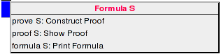
By selecting the menu entry "prove S" (or alternatively typing the command prove S; in the input field), the system switches from "declaration mode" to "proving mode" and start a proof of formula S. The screen now displays the content shown below:
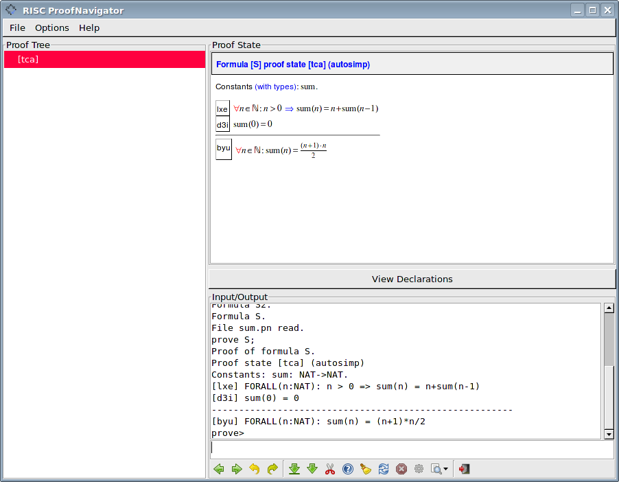
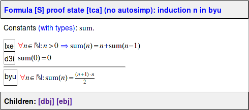
The proof consists of a single state with label [tca] which is indicated as the "current state" by the red line in the "Proof Tree" area. The three-character state label helps to uniquely identify a state within a proof; it is automatically generated and does not carry any meaning.
The "Proof State" area presents the state as2
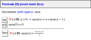
The presentation consists of the value constants visible in the state3 (sum) and of two sequences of labelled formulas: the assumptions (formulas [lxe] and [d3i]) and the goals (formula [byu]) separated by a horizontal line. The assumptions are obviously the contents of the axioms S1 and S2; the goal is the content of the formula S to be proved.
The logical interpretation of this presentation is that of a sequent; simply put our task is to prove that the conjunction of the assumptions (the formulas above the line) logically implies the disjunction of the goals (the formulas below the line). In our example, we thus have to prove that from the assumptions [lxe] and [d3i] the goal [byu] follows4.
A formula label consists typically of three characters that are automatically generated from the text of the formula (such that the same formula in different states has the same label) and does not carry any meaning. Formula labels are active elements; by moving the mouse cursor over a label, it turns blue and reveals a menu with a list of proof commands that are applicable to this formula. For instance, the following menu associated to goal [byu]
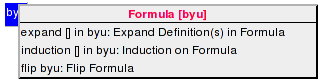
lists (among others) the command induction [] in byu which applies the proof technique of mathematical induction to formula [byu]; this formula must be a universally quantified formula with a variable from the domain of natural numbers. Actually, the menu entry is just a template with a parameter indicated by the token [] that has to be instantiated by the name of the variable on which to run the induction (in general, the quantifier may bind more than one variable). Selecting the template from the menu copies the template into the input area; the cursor is already placed on the parameter5 such that one just has to type the variable name n to get the full command
induction n in byu;
We might have typed in the command also directly on the command line; the formula menu just provided a convenient short-cut which saves us some typing effort (we will discuss later the various possibilities to enter a proof command). When the "Enter" key is pressed, the command is executed which updates the "Proof Tree" area to:
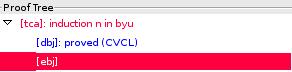
The original proof state [tca] is now labelled by the command "induction n in byu" applied in that state; furthermore it has received two children [dbj] and [ebj] which represent two proof obligations that replace the original obligation: the induction base and the induction step.
The induction base [dbj] was automatically proved by the external decision procedure CVCL which is indicated by the blue color and the comment "proved (CVCL)". Clicking on the corresponding line in the "Proof Tree" shows this already proved state in more detail:
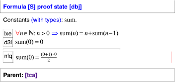
Apparently the new goal [nfq] is an instantiation of the original goal where the variable n is replaced by the constant 0 (a red bar is shown to the right of the goal to indicate that this is a formula that did not occur in the parent state). Since this goal is (after a bit of simplification) implied by the assumption [d3i], the system was able to prove it without human intervention.
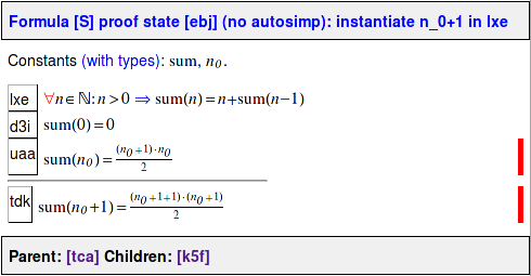
Clicking on the line with label [ebj] in the proof tree returns our focus to the proof state that actually requires our attention:
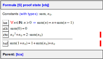
This state represents the induction step; it contains the declaration of a new natural number constant n0, an additional assumption [zkc] (representing the version of the original goal where the variable n is instantiated by n0) and a new goal [hsf] (representing the version of the original goal where the variable n is instantiated by the term 1+n0); red bars are shown to the right of these two formulas to indicate that they are new.
Actually, the system implicitly simplifies all formulas before it presents them to the user. Thus the formulas [zkc] and [hsf] are not syntactically equal but only logically equivalent to the instantiations
(1) sum(n_0)=(n_0+1)*n_0/2
(2) sum(1+n_0)=((1+n_0)+1)*(1+n_0)/2
of the original goal. While it is easy to see that formula [zkc] is derived from Equation (1) by simple arithmetic, it is not so easy to see that formula [hsf] is indeed equivalent to Equation (2). The derivation
sum(1+n_0) = ((1+n_0)+1)*(1+n_0)/2 = (n_0+2)*(n_0+1)/2
= (n_0^2+3*n_0+2)/2 = ((n_0^2+n_0)+2*n_0+2)/2 =(1) (2*sum(n_0)+2*n_0+2)/2
= sum(n_0)+n_0+1 = 1+sum(n_0)+n_0
shows that this is indeed the case under the assumption that Equation (1) holds (which is used in one step of the derivation). Such automatically performed transformations may help to considerably simplify a proof state, but their correctness may not always be immediately obvious to the user. Later we will also show a version of the proof with automatic simplification turned off.
In order to close the resulting proof state, we have to apply the knowledge contained in assumption [lxe]. By moving the mouse cursor over the label of this formula, a menu is revealed that shows us two possibilities to achieve this:
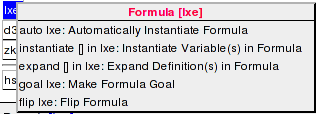
The menu entry for the command auto lxe promises an automatic instantiation of formula [lxe] while the entry for the command template instantiate [] in lxe asks for an explicit instantiation term for n. Although we may prefer the simpler auto lxe, it is in our example easy to see that the required instantiation term is n0+1 such that we may also select the template and instantiate it as follows:
instantiate n_0+1 in lxe;
(as one can see in the output area, the plain text form of n0 is n_0).
In either case (regardless of choosing auto or instantiate), the system prints in the output area
Proof state [k5f] is closed by decision procedure.
Formula S is proved. QED.
Proof saved (browse file S_index.xhtml).
Quit proof of formula S (use 'proof S' to see proof).
which indicates that formula S has been proved and that the system has returned to declaration mode. The menu of formula S is now
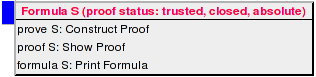
Its head line states that the formula has a proof with the following status: the proof is closed (it does not contain unproved states), trusted (it does not depend on declarations that have been changed since the proof was created), and absolute (it does not depend on other unproved formulas). Selecting the command proof S from the menu displays in the "Proof Tree" area the structure of this proof:
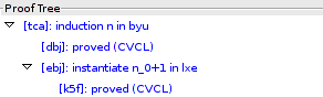
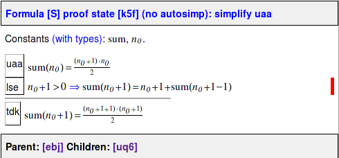
All proof states are shown in blue indicating the successful completion of the proof. We see that state [ebj] corresponding to the induction step is labelled by the command instantiate n_0+1 in lxe which has created a single child state [k5f]; clicking on this state shows its presentation in the "Proof State" area:
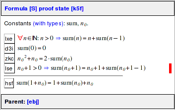
This state contains a single additional assumption [lse] representing the version of [lxe] where variable n is instantiated by the term n0+1. With the help of this assumption, the external decision procedure CVCL was able to close the proof state as indicated by the state comment "closed (CVCL)". If the command auto lxe is applied instead, the proof state contains a large number of automatically deduced instantiations, among them the one shown above.
As we have seen above, automatic transformations of formulas are handy but may sometimes be confusing. We may thus select the menu option "No Automatic Simplifications" which triggers the execution of the command
option autosimp="false";
which prevents in subsequently created proofs the automatic application of such simplifications (automatic simplification may be again switched on during a proof). We will now repeat above proof in this mode. We start by selecting in the menu of formula S the entry "prove S: Construct Proof" and then answer the question
Formula S already has a proof
  (proof status: trusted, closed, absolute)
Open existing proof (y/n)? n
by entering "n". This starts a new proof with the following root state:
The only difference to the root state of the previous proof is the annotation "no autosimp" which indicates that no automatic simplification is performed in the course of this proof. We again execute
induction n in byu;
which yields two child states. As before, the first state [dbj] representing the induction base is closed automatically. However, the second state [ebj] representing the induction step now looks as follows:
The formula [uaa] representing the induction hypothesis and the formula [tdk] representing the induction goal have not been simplified; they are exact copies of the original formula with the universally quantified variable n replaced by the values n0 and n0+1, respectively. If we now execute
instantiate n_0+1 in lxe;
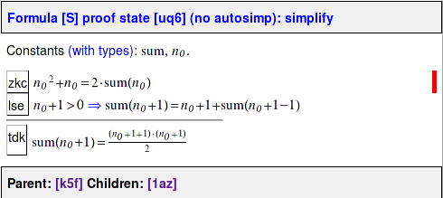
with get the proof state
where the formula [lse] is the instantiated version of [lxe] without further simplification. We may now select from the label menu of each formula, say [uaa], the entry "Simplify Formula"; this triggers the command simplify uaa which yields a new state [uq6] with the simplified formula [zkc]:
Alternatively, we may just press the button
![]() ("Simplify State") which triggers the
command simplify that simplifies all formulas in the current state
(as the default simplification mode always does): indeed, when we press this
button, the formulas are simplified in such a way that the external decision
procedure recognizes the goal as true and the proof state is closed.
("Simplify State") which triggers the
command simplify that simplifies all formulas in the current state
(as the default simplification mode always does): indeed, when we press this
button, the formulas are simplified in such a way that the external decision
procedure recognizes the goal as true and the proof state is closed.
Instead of pressing ![]() , we might have also chosen "Automatic
Simplification" from the "Options" menu to revert to the default
simplification mode (which would have also closed the proof state
immediately); by switching the automatic simplification mode selectively on
and off, different parts of a (bigger) proof may thus operate in different
modes.
, we might have also chosen "Automatic
Simplification" from the "Options" menu to revert to the default
simplification mode (which would have also closed the proof state
immediately); by switching the automatic simplification mode selectively on
and off, different parts of a (bigger) proof may thus operate in different
modes.
The software distribution contains in directory examples a text file sum.pn with the declarations given in this section and a subdirectory examples/sum with the proof as shown above. Rather than typing in the declarations manually, one may just go to examples, start the system and issue the command
read "sum.pn";
or just select the file from the GUI's menu entry "File/Read File". The system then reads the file, executes its declarations, and generates the output
read "sum.pn";
Value sum:NAT->NAT.
Formula S1.
Formula S2.
Formula S.
Proof read (proof status: trusted, closed, absolute).
File sum.pn read.
which indicates that the previously generated proof is now read from file. Actually, only a proof skeleton is read consisting of the commands performed to create the proof: while the proof tree may be still displayed by command proof S, clicking on the individual nodes of the tree only shows empty proof states. In order to re-generate also the states, the proof has to be replayed. This is achieved by simply executing the command prove S which will yield the following dialog:
prove S;
Formula S already has a (skeleton) proof
  (proof status: trusted, closed, absolute)
Replay skeleton proof (y/n)? y
Proof state [dbj] is closed by decision procedure.
Proof state [k5f] is closed by decision procedure.
Proof replay successful.
Use 'proof S' to see proof.
After typing "y" to the question "Replay skeleton proof (y/n)?", the system executes the proof commands while showing in the "Proof Tree" its progress. When the proof has been replayed, also the proof states can be displayed again.
The system keeps automatically track of the status of the declarations on which a proof depends; if some declaration has been changed since the time the proof was generated, the proof status is shown as "untrusted" which indicates that the proof replay might give errors. Replaying an untrusted proof resets its status to "trusted" (but possibly also from "closed" to "open", because some proof commands may yield errors such that some proof states cannot be closed any more). This automatic tracking of dependencies is a very helpful feature in the production of real-world proof where it is frequently the case that during the proof development some of the declarations change.
This first example should have given a first intuition about the style of interaction with the system. In the next section, we will illustrate more of its features by a more elaborate example.
| | 3.1 An Induction Proof |