Computing Factorial Numbers

4.1 Computing Factorial Numbers

In this section, we investigate the semantics and the verification of the program for computing factorial numbers already presented in Section 3.1:

  public static int fac(int n) /*@
    requires VAR n >= 0 AND factorial(VAR n) <= Base.MAX_INT;
    ensures VALUE@NEXT = factorial(VAR n);
  @*/
  {
    int i=1;
    int p=1;
    while (i <= n) /*@
      invariant VAR n >= 0 AND factorial(VAR n) <= Base.MAX_INT
            AND 1 <= VAR i AND VAR i <= VAR n+1
            AND VAR p = factorial(VAR i -1);
      decreases VAR n - VAR i + 1;
    @*/
    {
      p = p*i;
      i = i+1;
    }
    return p;
  }

Method Semantics

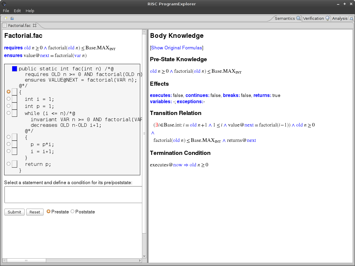
Right-clicking the item fac in the “Symbols” tree and selecting the menu entry “Show Semantics” lets the RISC ProgramExplorer switch to the “Semantics” view and display the information shown in Figure 4.1.

Figure 4.1.:

Semantics of Method fac (click to enlarge)

The view is split into several parts:

Method Definition: In the left pane, the definition of the method is shown with a column of active buttons (squares turning blue when the mouse is moved over them) to select the whole method body or an individual command of the body; additionally for each command a radio button is shown (see item “Condition Box” for their usage).
Statement Knowledge: In the right pane, all information derived from the analysis of the selected command is shown (see below for a detailed explanation of this information).
Condition Box: Below the method definition, a text box is shown. The user may select via the radio buttons to the left of the method body a single command, enter a state condition into the textbox, and fix this condition (via the two radio buttons below the box) to be either a “Prestate” or a “Poststate” condition. By pressing the button “Submit”, an additional view will be displayed that exhibits the effect of “pushing” the condition through the rest of the method body (we will later give an example).

In the pane “Bodsy/Statement Knowledge”, the following information is displayed for the selected method/command (which is also shown at the bottom of the pane):

Pre-State Knowledge

A condition which is known to hold whenever the command starts execution.

Effects

The effects that may be produced by the execution of the command.

Variables: The set of variables that may be modified by the command.
Exceptions: The set of exceptions that may be thrown by the command.
Executes: True, only if the command may terminate with the execution of a “normal” statement.
Continues: True, only if the command may terminate by executing continue.
Breaks: True, only if the command may terminate with the execution of break.
Returns: True, only if the command may terminate with the execution of return.

Transition Relation

The transition relation of the command, i.e., a formula describing the relationship between the pre-state and the post-state of the command execution.

Termination Condition

The termination condition of the command, i.e., a formula that describes a condition on the pre-state of the command execution which guarantees the termination of the execution.

By default, all formulas are shown after extensive logical simplification. By selecting the link “Show Original Formulas” the original formulas as constructed by the formal calculus are displayed (these are potentially huge but may be of interest if it is unclear how the simplified formula was derived).

For example, for the body of the method fac, the following information is derived:

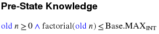
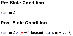
This is a copy of the method precondition.

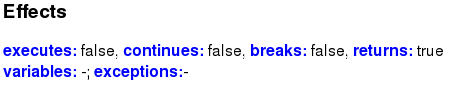
The method ends with a return statement and does not modify any global variable (all modified variables are local to the method).

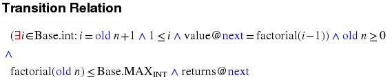
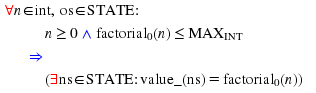
The core of this relation is the existential formula from which the formula value@next = factorial(old n) can be derived, i.e., the result of the function is the factorial of parameter n (the term value@next denotes the returned value in the post-state of the method execution). The remaining information drawn from the relation is that the original value of n must not be negative (old n ≥ 0), that the factorial of this value must not exceed the limit of type int (factorial(old n) ≤ Base.MAX_INT), and that the command always terminates with the execution of a return statement (returns@next).

The formula states that the method body terminates, if the original value of n is not negative (or that a predecessor command prevents the execution of the command, i.e., the pre-state of the command execution is not an “executing” one such that executes@now does not hold). This information is deduced from the fact that the value of the loop’s termination term must be initially non-negative.

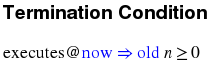
By selecting the body of the while loop, the following information is displayed:

We see from the pre-state knowledge that the body is only executed for 1 ≤ old i ≤ old n and that old p = factorial(old i-1); from the effects and the transition relation we can determine that the only effect of the body is to increment i and multiply p with (the old value of) i.

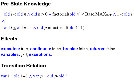
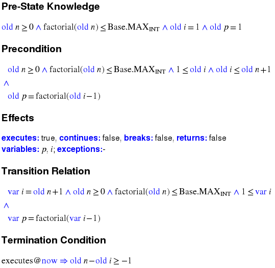
Selecting the whole loop, gives the following information:

We see from the pre-state knowledge that the loop is executed with old n ≥ 0 and old i = 1; from this and the termination condition old n-old i ≥-1, the termination of the loop can be established. The transition relation also tells us that var i = old n+1, i.e., that the loop terminates with the value of i being n+1 (since from the effects we know that n is not changed); from this and var p = factorial(var i-1), we know that the loop terminates with p being factorial(n).

We may also the investigate the effect of imposing additional constraints on certain states. For example, we may select with the radio button the body of the while loop and enter into the textbox as a “Prestate” condition

VAR i=2

After pressing the “Submit” button, we get the view depicted in Figure 4.2.

Figure 4.2.:

Constraining a State (click to enlarge)

The green marker indicates for which statement the condition has been fixed that is indicated at the bottom of the left pane. By moving the mouse over the markers we may investigate the effects of this constraint for selected statement. For instance, when selecting

p = p*i;

we get the information

When selecting

i = i+1;

we get

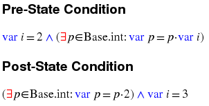
i.e., we know that after the execution of the loop body p is even and i equals 3.

Method Verification

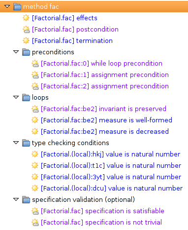
After the investigation of the method semantics (which has not given any indication of a problem so far), we may turn to the actual verification of the method. We return to the “Analysis” view and investigate the task tree of the method which is displayed in Figure 4.3 (some of the tasks labeled in violet may also be labeled red, if the corresponding proof has not yet been performed). Open tasks are indicated by red task labels.

Figure 4.3.:

Verification Tasks (click to enlarge)

The solution of a task proceeds by

translating the task to a “state proving problem” in the language of the RISC ProgramExplorer (such a problem may include built-in state predicates that are not part of classical logic), then
translating the state proving problem into a “classical proving problem” in the language of the RISC ProgramExplorer (the built-in state predicates have been translated to defined predicates), and finally
translating the classical proving problem into a “ProofNavigator problem”, i.e. a problem in the language of the RISC ProofNavigator (which is slightly different from that of the RISC ProgramExplorer).

By right-clicking the symbol of an open task, a menu appears that allows to print the corresponding task translations in a linear format (this is mainly useful to investigate how the final proof problem was generated from the original task).

For solving the proof problem associated to an open task, there exist three options:

For certain tasks, the built-in validity checker is automatically applied to the problem; if it is successful, the task label turns blue immediately.
Otherwise (the validity checker does not succeed or is not even attempted due to minor chances of success), a proof is required. Such a proof is started by right-clicking a task symbol and selecting “Execute Task”. Then the automatic scatter strategy is applied; if it is successful, the task label turns blue.
Otherwise (the scatter strategy does not succeed), an interactive proof is started. The RISC Program Explorer switches to the “Verification” view which is essentially the interface of the RISC ProofNavigator. This view is left by pressing the button Quit Proof (after confirmation); if the proof has been completed, the task label turns blue, otherwise it stays red.

In the last two cases, a proof is generated and stored on disk. If the RISC ProgramExplorer is terminated and restarted, the labels of the corresponding tasks are displayed in violet color. On performing “Execute Task”, the stored proof is replayed and the label turns blue again.

In detail, the following tasks need to be performed:

Effects

This is the task to show that the method only modifies those global variables that are indicated in the modifies clause of the method header. This task can be automatically performed by the implemented calculus¹ .

Postcondition

This is the task to show the partial correctness of the method, i.e. that the method ensures the postcondition indicated in the ensures clause of the method header. No attempt is made to apply the validity checker; there is always a proof required.

Termination

This is the task to extend the partial correctness of the method to its total correctness, i.e. to show that the method also terminates. It is first attempted to solve the task by the validity checker before a proof is requested.

Measure

For a recursive method, this is the task to show that the method measure is well-formed, i.e. that the method precondition implies that the method measure is not negative (the fact that the measure is decreased by a recursive call is proved as part of the caller method’s termination condition).

Preconditions

Each statement (such as an assignment) may be only executed, if the statement’s precondition is satisfied (e.g. that the evaluation of an expression that occurs in the statement does not yield an arithmetic overflow). For every statement with a non-trivial precondition, a task is generated to show that the precondition is ensured when the statement is executed. It is first attempted to solve the task by the validity checker before a proof is requested.

Loops

For each loop (for or while loop), several tasks are generated:

Invariant is preserved: This is the task to show that the invariant is preserved by the execution of the loop body (the fact that the invariant initially holds is added to the loop’s precondition). No attempt is made to apply the validity checker; there is always a proof required.
Body terminates: This is the task to show that the execution of the loop body terminates. The validity checker is applied before a proof is requested.
Measure is well-formed: This is the task to show that the value of the termination term does not become negative² by any execution of the loop body (the fact that the value of the termination term is initially not negative is shown as part of the enclosing method’s termination condition). The validity checker is applied before a proof is requested.
Measure is decreased: This is the task to show the value of the termination term is decreased by every execution of the loop body³ . The validity checker is applied before a proof is requested.

Type-checking Conditions

Most aspects of a formula’s type correctness can be verified by a static calculus, some aspects (such that in a particular occurrence of a term x/y the variable y is not negative) give rise to verification tasks. Most of these tasks can be performed by the validity checker; in some cases, however, a proof is requested.

Specification Validation (Optional)

The software also generates two conditions whose proofs are not mandatory but which may/should be performed before proceeding with the rest of the verification.

It should be shown that a “specification is satisfiable”, i.e., that for every pre-state value that satisfies the method’s precondition there exists a post-state value that satisfies the postcondition. If a specification is not satisfiable, every attempt to verify partial correctness is a priori doomed.
It should be shown that a “specification is not trivial”, i.e., that for every pre-state value that satisfies the method’s precondition there exists a post-state value that does not satisfy the postcondition. If a specification is trivial, it indicates that every implementation is legal, which is a strong hint that the specification is flawed.

No attempt is made to apply the validity checker; there is always a proof requested.

The tasks are partially interdependent, e.g., the proof of partial correctness (performed in task “postcondition”) depends of the fulfillment of tasks “preconditions” and of the “loops”. However, the tasks can be performed in any order, e.g. it is recommended to first solve the “postcondition” task (under the assumption that the invariants hold) and only afterward solve “loops” (which are typically more difficult). In this way, no time is wasted on proving the correctness of an invariant that is not strong enough to show the partial correctness of a method.

In the following, we investigate the tasks for the method fac in some more detail.

Postcondition For a method with precondition p and state relation r, to show that the postcondition q is satisfied amounts to proving

p∧r ⇒ q

(logically equivalent to r ⇒ (p ⇒ q)). Here p and q are part of the method header (requires p ensures q) and r is shown in the Semantics view of the method (“State Relation”).

In our case, we have to prove

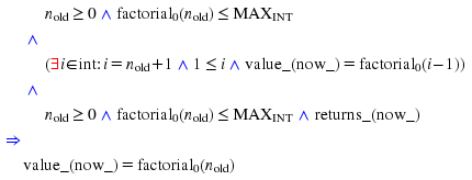
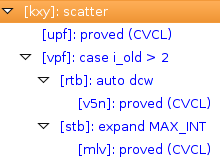
where the first line corresponds to p, the next two lines correspond to r, and the last line corresponds to q. The proof succeeds by the automatic scatter strategy.

Termination The proof that the “method body terminates” is of form

p∧¬d ⇒ t

where p represents the precondition of the method, d represents the diverges condition in the method’s specification (an optional condition under which the method is allowed to run forever) and t is the loop body’s termination condition (as depicted in the “Semantics” view of the method).

In our case, the termination condition is essentially old n ≥ 0 which is part of the pre-condition; the corresponding task is solved by the validity checker.

Preconditions For a command with pre-state knowledge k and pre-condition c, to show that the pre-condition is met amounts to proving

k ⇒ c

where both k and c are displayed in the Semantics view of the method (“Pre-State Knowledge” and “Precondition”).

In our example, there are three precondition tasks, one for the loop (to show that the loop invariant initially holds), the other two for the assignments and in the loop body (to show that no arithmetic overflows occur). The first proof of

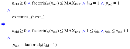
is (after triggering the proof) solved automatically. The second proof of

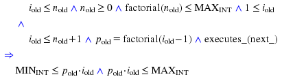
(which correspods to the assignment p = p*i) requires some arithmetic reasoning with the help of additional lemmas about the factorial function specified in theory Math; we omit it here. The third proof of

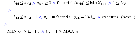
(which corresponds to the assignment i = i+1) is simpler; it only depends on the theorem ∀n ∈ NAT : n > 2 ⇒ factorial(n) > n; the corresponding proof tree is

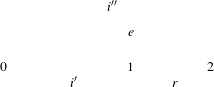
Loops For a while loop with invariant i and a body with state relation r, the proof of the correctness of the invariant amounts to proving a formula of form

i′∧e∧r ⇒ i′′

Here i′ represents a variant of i that expresses the relationship between the initial state 0 of the loop and the state 1 before the current loop iteration, e expresses the fact that the loop condition holds at state 1, r expresses the relation between the states 1 and 2 before and after the current loop iteration, and i′′ represents a variant of i that expresses the relationship between states 0 and 2:

PICT PICT

In our example, this amounts to proving (after some simplification) the formula

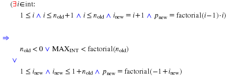
This corresponding proof tree is

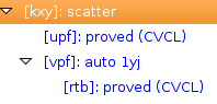
i.e., the proof requires the heuristic instantiation of formula “1yj” which represents the factorial axiom ∀n ∈ NAT : factorial(n+1) = (n+1)⋅factorial(n).

The proof that the loop “body terminates” is essentially to show

i′∧e ⇒ b

where i′ and e are as indicated above and b is the condition for the termination of the loop body.

In our case, b is true such that the corresponding task is not generated.

The proof that the loop “measure is well-formed” is essentially to show

i′∧e∧r ⇒ t′≥ 0

where i′, e, and r are as indicated in the paragraph “Invariants” above and t′ represents the value of the termination term after the loop iteration.

In our case, t′ is denoted by old n-var i+1 where e represents old i ≤ old n and r implies var i = old i+1; the corresponding task can be solved by the validity checker.

The proof that the loop “measure is decreased” is essentially to show

i′∧e∧r ⇒ t > t′

where i′, e, r, and t′ are indicated as above and t represents the value of the termination term before the iteration of the loop.

In our case, t is denoted by old n- old i+1 with the other definitions given above; the corresponding task can be solved by the validity checker.

Type Checking Conditions The type checking conditions all result from the fact that in the method specification respectively loop invariant terms like factorial(var n) respectively factorial(var i-1) occur; for each such occurrence it has to be shown that the argument of factorial : NAT → NAT (which is by static type checking known to be an integer number) is a natural number, i.e., not negative. All the corresponding tasks can be automatically solved by the validity checker.

Specification Validation The validation of a method specification with precondition p and postcondition q amounts to proving

∀x : p(x) ⇒∃y : q(x,y)
∀x : p(x) ⇒∃y : ¬q(x,y)

where x represents the pre-state of the method (containing method arguments etc) and y represents its post-state (containing the method result); we thus show that for every legal input there exists some legal output (the specification is satisfiable) and some output that is not legal (the specification is not trivial).

In case of the method fac, this amounts to proving the following:

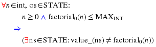
The corresponding proof trees are as follows:

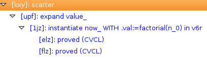
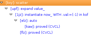
The proof for satisfiability amounts to instantiating, for given method argument n₀, the existential formula with a poststate derived from the prestate “now_” by setting the return value to factorial(n₀); in the proof of non-triviality, the return value is set to -1 (a state, i.e. a value of type “STATE”, is a record whose field val denotes the state’s return value, if there is any).

[next] [front] [up]