, enter the file name Math.theory,
and press Okay. In the central region a new editing area titled Math.theory opens; we enter above
theory declaration and press the button Save File
, enter the file name Math.theory,
and press Okay. In the central region a new editing area titled Math.theory opens; we enter above
theory declaration and press the button Save File  . The RISC ProgramExplorer window has
then the state shown below:
. The RISC ProgramExplorer window has
then the state shown below: This example is about the specification of the following program
The program is written in Java-syntax; it introduces a method fac which is supposed to return the factorial of its argument n.
The specification of the program is to be based on the mathematical function factorial : NAT → NAT which is uniquely characterized by the axioms
factorial(0) = 1
∀n ∈ NAT : factorial(n+1) = (n+1)⋅ factorial(n)
First we describe how to define the corresponding mathematical theory, next we describe how to specify the program with the help of this theory.
Theory We define a theory Math which introduces a function factorial on the natural numbers and constrains its behavior by two axioms as discussed above and also contains a logical consequence of these axioms:
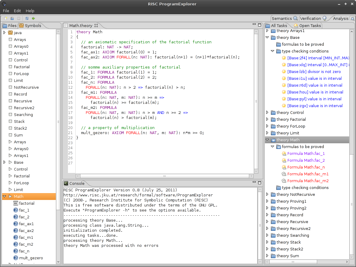
We can use the RISC ProgramExplorer to write this theory in a file Math.theory in the unnamed
top-level package as follows: we select the button New File , enter the file name Math.theory,
and press Okay. In the central region a new editing area titled Math.theory opens; we enter above
theory declaration and press the button Save File . The RISC ProgramExplorer window has
then the state shown below:
The theory is displayed as
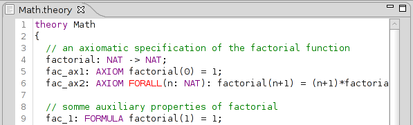
with colors indicating keywords of the specification language. Identifiers are active, e.g. by double-clicking on factorial the identifier is highlighted, the tab Symbol on the left side of the window highlights the corresponding symbol and the Console area displays
(likewise the identifiers Math, fac_1, and fac_2 can be double-clicked). Moving the mouse pointer over the symbol on the left tab displays a corresponding yellow “tip” window, clicking with the right mouse-button allows to choose between Print Symbol and Print Declaration. Choosing the symbol Math and selecting Print Symbol displays in the console area output similar to
Selecting Print Declaration displays
If we introduce in the declaration an error, e.g. by mistyping the function name as factorials in axiom
the Console area shows the output
In the editing area, the theory is then displayed as
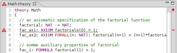
The position of the error in the file is indicated by an icon  on the left bar, by a
corresponding red marker on the right bar and by underlining the syntactic phrase in red; moving
the mouse pointer over the icon on the left or over the marker on the right displays the
corresponding error message. The same icon at the top of the editing tab and in the tab
Symbols indicates that the theory has an error. Moving the mouse pointer over the red
square on the top-right corner of the editing area displays the number of errors in the
theory. After fixing the error and pressing the button Save File , the correct state is
restored.
on the left bar, by a
corresponding red marker on the right bar and by underlining the syntactic phrase in red; moving
the mouse pointer over the icon on the left or over the marker on the right displays the
corresponding error message. The same icon at the top of the editing tab and in the tab
Symbols indicates that the theory has an error. Moving the mouse pointer over the red
square on the top-right corner of the editing area displays the number of errors in the
theory. After fixing the error and pressing the button Save File , the correct state is
restored.
The tab All Tasks on the right now contains the following entries:
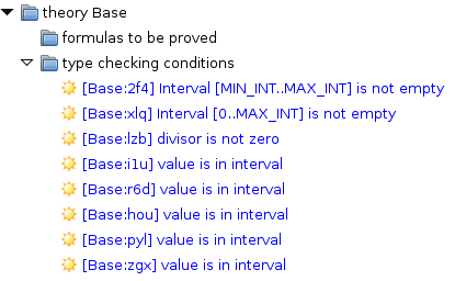
The folder theory Base contains a subfolder type checking conditions which holds those tasks that arose from type-checking a built-in “base” theory. The task labels shortly describe the tasks; the automatically generated tags of the form [Base:ccc] allow unique referencing; the blue font indicates that all the tasks could be performed with the help of an automatic strategy. Moving the mouse pointer over the tasks (respectively right-clicking the tasks and selecting the option Print Task) shows the task descriptions, e.g.
The special icon  indicates that it contains (subfolders with) open tasks to be performed.
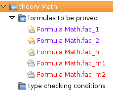
Indeed it contains a subfolder formulas to be proved with some open tasks labeled in red referring to
formulas that have not yet been proved. The icon
indicates that it contains (subfolders with) open tasks to be performed.
Indeed it contains a subfolder formulas to be proved with some open tasks labeled in red referring to
formulas that have not yet been proved. The icon  indicates that the corresponding task is
“new”, while the icon
indicates that the corresponding task is
“new”, while the icon  indicates that the task has a previously constructed proof attempt
(i.e. an incomplete proof that may be replaced and completed in the current invocation). On the other
hand, those tasks with icon and violet labels are already closed; they refer to formulas that
have been proved in a previous invocation such that the proofs may be simply replayed in the current
invocation.
indicates that the task has a previously constructed proof attempt
(i.e. an incomplete proof that may be replaced and completed in the current invocation). On the other
hand, those tasks with icon and violet labels are already closed; they refer to formulas that
have been proved in a previous invocation such that the proofs may be simply replayed in the current
invocation.
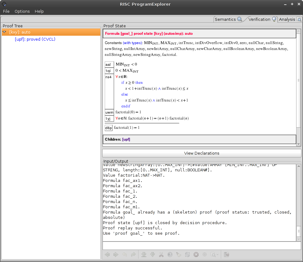
Right-clicking any of these tasks and selecting the option Print Classical Proving Problem shows the detailed proofs to be performed for performing the tasks: in the case of “Formula fac_1”, this proof is
Right-clicking the task and selecting the option Execute Task replays the (simple) previously constructed proof; selecting the option Show Proof displays the view shown below:
This is essentially a view on the RISC ProofNavigator [8, 5], the computer-assisted interactive proving assistant integrated into the RISC ProgramExplorer. The task generated by the RISC ProgramExplorer was translated into a proving problem of the RISC ProofNavigator and performed with human aid (in this case, by invoking the auto command for heuristic instantiation of quantified formulas). By clicking on the individual nodes of the proof tree shown to the left, the corresponding proof situations are displayed; pressing the button View Declarations displays the declarations related to the proof. By selecting the tab “Analysis” we return to the original view. Right-clicking the task and selecting “Reset Task” resets the task to its original “new” state (deleting the previously constructed proof) such that a fresh interactive proof attempt can be performed.
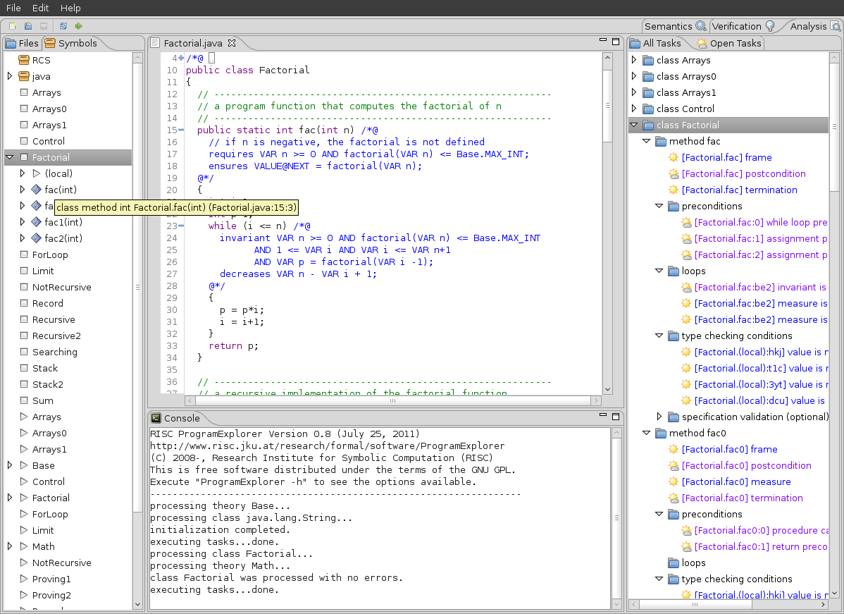
Program We can now create (in analogy to file Math.theory) a program file Factorial.java which holds the program class Factorial described above. Saving the file type-checks it and creates in tab Symbols a class symbol Factorial with method symbol fac and parameter symbol n. As for theories, also the identifiers in the source file are active, double-clicking e.g. on fac in the editing area prints the method declaration in the Console area and highlights the symbol fac in the Symbols tab. Correspondingly, double-clicking the symbol fac moves the editor to the position of the declaration of the method and highlights its header.
To formally specify the behavior of the method fac with the help of the theory Math, we annotate the class Factorial by special program comments /*@ …@*/ as follows:
The RISC ProgramExplorer window has then the state shown below:
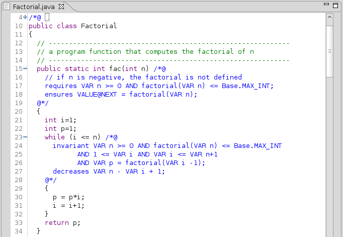
The actual program code is displayed as shown below:
Annotations can become “folded” away from the program source code; clicking on the icon
 folds the annotation, clicking on the icon
  unfolds it again. Moving the mouse
pointer over the icon displays the content of the folded annotation in a yellow “tip”
window.
unfolds it again. Moving the mouse
pointer over the icon displays the content of the folded annotation in a yellow “tip”
window.
The annotation theory … before the class declaration introduces the “local” theory for the class i.e. those entities that may be further on referenced by short names; the uses Math clause indicates that the local theory refers to entities of the previously defined theory Math. The local theory is simple: it just defines a function factorial by the corresponding function in theory Math which can be referenced by the long name Math.factorial. Alternatively, we might have referred in the following directly to Math.factorial (however, even then an empty declaration theory uses Math { } is required because we refer to theory Math) or we might have just axiomatized the function factorial directly in the local theory (without referring to theory Math at all).
The annotation requires …ensures … after the header of method fac introduces a method specification by a precondition (requires …) that describes the assumptions on the prestate of the method call (in particular constraints of the method arguments) and a postcondition (ensures …) that describes the obligation on the poststate of the method call (in particular obligations on the method result). In our case, the precondition
states that the value of the program variable n (the method parameter) indicated by the term VAR n must not be negative when the method is called and that the value of factorial(n) must not exceed the limit of the program type int indicated by the mathematical constant MAX_INT in the base theory. The postcondition
states the method result indicated by the term VALUE@NEXT must be identical to the value of the logical function factorial when applied to the value of n.
Finally, the body of the while loop is annotated by a loop invariant and a termination term: the loop invariant essentially states the relationship of the prestate of the loop to the poststate of every iteration of the loop body; the termination term denotes a non-negative integer number that is decreased by every iteration of the loop. In our case, the invariant
limits the range of the iteration counter i and states that the value of the program variable p is identical to the factorial of the value of i. The termination term
states that the value of i is decremented by every loop iteration but does not become bigger than n+1.
Type-checking the annotations and semantically processing the class gives rise to a number of tasks in folder class Factorial organized in a couple of subfolders (as usual double-clicking on the tasks highlights the corresponding source code positions; moving the mouse over the tasks shows their description). The folder type checking conditions contains those tasks arising from type checking the annotations; all of them can be closed by an automatic strategy. The other conditions refer to the correctness of the method with respect to its specification; they will be discussed in Chapter 4.