![c : [f]xs x ⁄∈ xs
-----------g,h--------xs ∪-{x}
c : [f ∧ var x = old x]g,h](main2x.png)
![---------e ≃h-t--------
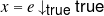
x = e : [var x = t]{trxu}e,h](main3x.png)
![c : [f ]xgs,h
------------------------------------------xs\x----------
{var x; c} : [∃x0,x1 : f[x0∕old x,x1∕var x]]g,∀x:h[x∕oldx]](main4x.png)
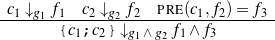
![c1 : [f1]xgs,h c2 : [f2]xgs,h PRE (c1,h2) = h3
-{c--;c-}-: [∃1ys1 : f-[ys∕var-xs2]∧2f-[ys∕old-xs]]xs--------
1 2 1 2 g1∧g2,h1∧h3](main5x.png)
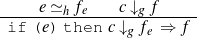
![e ≃ f c : [f ]xs
-------------------h-e----------------1---1g1,h1---------------
if (e) then c : [if fe then f1 else var xs = old xs]xgs1,h ∧(fe ⇒ h1)](main6x.png)
![e ≃h fe c1 : [f1]xgs,h c2 : [f2]xgs,h
------------------------------------1--1-------xs---------2-2-----------
if (e) then c1 else c2 : [if fe then f1 else f2]g1∧g2,h∧iffe then h1 elseh2](main7x.png)
![xs
e ≃h fe c : [fc]gc,hc
g ≡ ∀xs,ys,zs : f[xs∕old xs,ys∕var xs]∧ fe[ys∕old xs]∧ fc[ys∕old xs,zs∕var xs] ⇒
h[ys∕old xs]∧ f[xs∕old xs,zs∕var xs]
---------while---(e)f,t c-: [f-∧-¬f-[var-xs∕old-xs]]xs--------------------------
e gc∧ g,h ∧f[old xs∕varxs]](main8x.png)
| Figure A.1.: | The Transition Rules |
In this chapter (whose material is based on [9]), we sketch the formal calculus on which the RISC ProgramExplorer is founded. To simplify the presentation, we do not refer to the subset of Java which is actually used in the software but to a simple command language without control flow interruptions and method calls. In this language, a command c can be formed according to the grammar
c ::= x = e | {var x; c} | {c1;c2}
| if (e) then c | if (e) then c1 else c2 | while (e)f,t c
where x denotes a program variable, e denotes a program expression, and a while loop is annotated by an invariant formula f and termination term t. The semantics of a command c is defined, for a given set Store of possible states (store contents), by a binary relation ⟦c⟧ ⊆ Store × Store that defines the possible state transitions of the command and by a set ⟨⟨c⟩⟩⊆ Store that defines those pre-states where the command must perform a transition to some post-state; for a definition of the semantics, see [6].
In Figures A.1, A.2, and A.3, we give rules (where the terms old xs and var xs refer to the sets of values of the program variables xs in the pre-/post-state) to derive for the commands shown above the following three kinds of judgments:
The derivations make use of additional judgments e ≃fef and e ≃fet which translate a boolean-valued program expression e into a logic formula f and an expression e of any other type into a term t, provided that the state in which e is evaluated satisfies the condition fe (the rules for these judgments are omitted).
One should note that the rules presented in Figures A.1 and A.2 can be applied recursively over the structure of a command; first we determine the transition/termination formula of the subcommands, then we combine the formulas to the transition/termination formula of the whole command. Along this process, the side condition h is constructed which has to be shown separately to hold in the pre-state of the command in order to verify the correctness of the translation.
A special case is the rule for while loops. Here the result is only determined by the invariant formula respectively termination term by which the loop is annotated; additionally, a proof obligation g is generated to verify the correctness of the loop body with respect to invariant and termination term. In a similar way, in the full programming language calls of program methods are handled: the transition relation of the method call is derived from the specification of the method; the correctness of the implementation of the method is to be established separately. We thus yield a modular approach to the derivation of transition relations and termination conditions; the size of the derived formula is independent of the sizes of the bodies of the loops executed respectively of the methods called. Furthermore, the approach gives rise to some sort of “correct by construction” approach: we may first develop loop invariants and method preconditions (and verify the correctness of programs executing the loops and calling the methods) before we implement the bodies of the loops and methods (and consequently verify the correctness of implementations).
Formally, the derivations satisfy the following soundness constraints.
Theorem 1 (Soundness) For all c ∈ Command, fr,fc,fp,fq,g,h ∈ Formula, and for all xs ∈ ℙ(Variable), the following statements hold:


The semantics ⟦f ⟧(s,s′) of a transition relation f is determined over a pair of states s,s′ (and a logic environment, which is omitted for clarity); the semantics of state condition g is defined as ⟦g⟧(s) ⇔∀s′ : ⟦g⟧(s,s′) and the semantics of a state independent-condition h is defined as ⟦h⟧ ⇔∀s,s′ : ⟦h⟧(s,s′).
In [7], the formal semantics of commands and formulas has been defined and the soundness of (a preliminary form of) the calculus has been proved. In [6], a concise definition of the semantics, judgments, and rules of (an older form of) the calculus is given.
![------------c-↓g-f------------
{var x; c} ↓g ∀x : f[x∕old x ]](main10x.png)

![e ≃ f c : [f ]xs c ↓ f
h e c gc,hc gt t
g ≡ ∀xs,ys,zs : f[xs∕old xs,ys∕var xs]∧ fe[ys∕old xs]∧ fc[ys∕old xs,zs∕var xs] ⇒
-----------------ft[ys∕old xs]∧-0-≤-t[zs∕old-xs] <-t[ys∕old xs]---------------
while (e)f,t c ↓g∧ g t ≥ 0
t](main14x.png)
![c : [f ]xs
------------------------g,h-------------------
PRE (c,fq) = ∀ xs : f[xs∕var xs] ⇒ fq[xs∕old xs]](main15x.png)
![xs
--------------------------c : [f]g,h------------------------
POST (c,fp) = ∃xs : fp[xs∕old xs]∧ f[xs∕old xs,old xs∕var xs]](main16x.png)