7.3 Graphs
Basic Notions
Throughout this document, we have used graphs as visual illustrations of
binary relations. However, we can also consider graphs themselves as
mathematical objects that are represented by binary relations. The theory of
graphs has many applications in various scientific areas; they can be used to
model railroad plans as well as electrical circuits, molecules as well as
brain structures.
Definition 123 (Directed Graph)
A directed graph (gerichteter Graph) is a pair <V,
E> of a set V of vertices (Knoten) or nodes and
a set of E of edges (Kanten) or arcs where E is
a binary relation on S:
|
G is directed graph : <=> |
|
exists V, E: |
|
G = <V, E> /\ |
|
E subset V x V.
|
An element <x, y> in E expresses the fact
that node x is connected to node y where x is called the
initial node of the corresponding edge and y is called its
terminal node. Both nodes are then adjazent.
Please note that in above definition of a graph there may be at most one edge
between any pair of nodes. A graph with potentially more than one edge between
two nodes is called a multigraph (Multigraph) which may be used to
describes e.g. multiple roads between two cities. Furthermore, the edges in a
graph may be labelled with real values; such a graph is called a
weighted graph (gewichteter Graph) and may describe lengths of roads or
capacities of water pipes. However, we will not consider the formalization of
such graphs in this document.
Example
The matrix representation of a graph used in above example can be
formalized as follows.
Definition 124 (Adjacency Matrix)
Let G = <V, E> be a directed graph with
|V| = n. The adjacency matrix (Adjazenzmatrix,
Nachbarschaftsmatrix) of G is the boolean n * n matrix
M where M(x, y) = true if and only if
<x, y>
in E:
|
adjacency(G) := |
|
let V = G0, E = G1:
|
|
such M in V x V -> {true, false}: |
|
(forall x in V, y in V: M(x, y) = true <=> <x, y> in E).
|
The adjacency matrix is the typical implementation of a graph in a computer;
most graph algorithms operate with this representation.
Example
Let R and S be binary relations on Nn for some
n in N. The composition of R and S is
|
R o S = {<a, c>: a in Nn /\ c in Nn /\ (exists b: <a, b> in R /\ <b, c> in S)}.
|
For the corresponding adjacency matrix, we thus have
|
forall i in Nn, j in Nn: |
|
adjacency(<Nn, R o S>)i, j =
true <=> |
|
exists k in Nn: Ai, k =
true /\ Bk, j = true |
|
where A = adjacency(<Nn, R>), B =
adjacency(<Nn, S>).
|
Written as a Java method, the composition of two adjacency matrices A
and B giving a result matrix C resembles
matrix multiplication:
void compose(int n, boolean[][] A, boolean[][] B, boolean[][] C)
{
  for (int i=0; i<n; i++)
    for (int j=0; j<n; j++)
    {
      C[i][j] = false;
      for (int k=0; k<n; k++)
        C[i][j] = C[i][j] || (A[i][k] && B[k][j]);
    }
  return C;
}
In some graphs, the direction of the edges does not matter.
Definition 125 (Undirected Graph)
An undirected graph (ungerichteter Graph) is a directed graph whose
edge relation is symmetric:
|
G is undirected graph : <=> |
|
exists V, E: |
|
G = <V, E>, |
|
E subset V x V, |
|
E is symmetric on V. |
|
|
According to this definition, an undirected graph is a special directed graph;
therefore all the following definitions and results for directed graphs apply
to undirected graphs as well. Because of symmetry, the only information
carried by an undirected graph is whether two nodes x and
y are connected or not; in the visual representation it suffices to
draw a single undirected edge between two connected nodes.
Example
- The graph <N_5, E> with
|
E = {<0, 1>, <1, 0>, <0, 2>, <2, 0>,
<1, 1>, <1, 2>, |
|
<2, 1>, <3, 3>, <0, 4>, <4, 0>, <1, 4>,
<4, 1>}
|
can be depicted as follows:
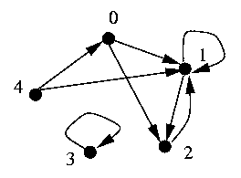
We just need to fill the elements of the upper right triangle of the matrix
representation; the other elements are determined by symmetricity:
|
| 0 | 1 | 2 | 3 | 4 |
|
0 | false | true | true | false | true |
|
1 | | true | true | false | true |
|
2 | | | false | false | false |
|
3 | | | | true | false |
|
4 | | | | | false
|
- The graph <{a, b, c},
E> with
|
E = {<a, a>,
<a, b>, <b, a>}
|
can be depicted as

and has the following matrix representation:
|
| a | b | c |
|
a | true | true | false |
|
b | | false | false |
|
c | | | false |
|
|
An important notion is the number of edges that enter or leave a node.
Definition 126 (Degree)
In a directed graph, the indegree (eingehender Grad) of x is the
number of edges whose terminal node is x:
|
indegG(x) := |{y in V: <y, x> in E}| |
|
where V=G0, E=G1.
|
The outdegree (ausgehender Grad)
of x is the number of edges whose initial node is x:
|
outdegG(x) := |{y in V: <x, y> in E}| |
|
where V=G0, E=G1.
|
The total degree (Grad) of x is the sum of its indegree and its
outdegree:
|
degG(x) := indegG(x) +
outdegG(x).
|
Example
- In the graph

the indegree of node 1 is 4 and its outdegree is 2.
- In the graph

the indegree and the outdegree of node c are both 0.
Applied to undirected graphs, above definition makes the indegree of a node
equal its outdegree and the total degree be even; since in undirected graphs
the only interesting information is the total degree, this number is then
usually divided by two in correspondence with the visual representation.
Even if two graphs are different, they may have the same structure.
Definition 127 (Graph Isomorphism)
Two graphs are isomorphic (isomorph) if there exists a
bijection between the nodes of the two graphs which preserves the edge
structure:
|
G and G' are isomorphic : <=> |
|
G is directed graph /\ G' is directed graph /\ |
|
exists f: f: V ->iso(E, E')
V' |
|
where V = G0, E = G1, V' =
G'0, E' = G'1.
|
Example
- The graphs
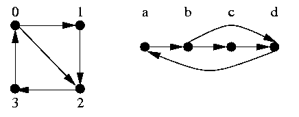
are isomorphic with isomorphism
|
f = {<0, b>, <1, c>, <2,
d>, <3, a>}.
|
- The graphs
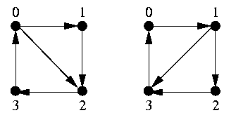
are isomorphic with isomorphism
|
f = {<0, 1>, <1, 2>, <2,
3>, <3, 0>}.
|
- The graphs
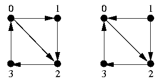
are not isomorphic.
The edges of a node yield paths that can be used to wander among nodes.
Definition 128 (Path)
A path (Pfad) in a graph is a sequence of nodes connected by edges:
|
p is path in G : <=> |
|
(exists n in N>0:
p: Nn -> V /\ |
|
forall i in Nn-1: <pi, pi+1> in E) |
|
where V=G0, E=G1.
|
The length (Länge) of a path is the number of edges
it contains:
|
length(p) := such n in N: p:
Nn+1 -> V.
|
A path from x to y has initial node
x and terminal node y : <=> |
p is path from x to y : <=> |
|
p0 = x /\ pn = y |
|
where n = length(p).
|
A path is simple (einfach) if it does not contain any edge twice:
|
p is simple : <=> |
|
forall i in Nn, j in Nn: <pi, pi+1> =
<pj, pj+1>
=> i = j |
|
where n = length(p).
|
A path is elementary (elementar) if it does not contain any node twice:
|
p is elementary : <=> |
|
forall i in Nn, j in Nn: pi =
pj => i = j |
|
where n = length(p).
|
A path is a cycle (Kreis) or circuit if it terminates in its
initial node:
|
p is cycle : <=> exists x: p
is path from x to x.
|
Reachability We will now investigate how to determine whether
two nodes are directly or indirectly connected in a graph.
Definition 129 (Reachable)
A node y is reachable (erreichbar) from a node x in a
graph G if there is a path in G from x to y:
|
y is reachable from x in G
: <=> |
|
exists p:
p is path in G /\ p is path from x to y.
|
The predicate "is reachable" is, for fixed graph G=<V,
E>, a binary relation on V, as well as the edge relation
E is. Actually we can derive from E the reachability relation
by a general construction that we are going to elaborate.
Definition 130 (Reflexive and Transitive Closure)
Let R be a binary relation on S.
The reflexive closure (reflexiver Abschluß) of R on S
is the smallest relation that contains R and is reflexive on S:
|
reflexiveS(R) := |
|
such R' subset S x S: |
|
R subset R' /\ R' is reflexive on
S /\ |
|
forall R": (R subset R" /\ R"
is reflexive on S) => R' subset R".
|
The transitive closure (transitiver Abschluß) of R on S
is the smallest relation that contains R and is transitive on S:
|
transitiveS(R) := |
|
such R' subset S x S: |
|
R subset R' /\ R' is transitive on
S /\ |
|
forall R": (R subset R" /\ R"
is transitive on S) => R' subset R".
|
We then can derive the following result.
Proposition 131 (Reachability is Closure of Edge Relation)
We define the reachability relation
|
RG := {<x,
y> in G0 x G0: y
is reachable from x in G}.
|
Then, for any directed graph <V, E>,
R<V, E> is
the reflexive and transitive closure of E on V:
|
forall V, E: <V, E>
is directed graph => |
|
R<V, E> =
reflexiveV(transitiveV(E)).
|
Example
Take the graph <N_5, E> with
|
E = {<0, 1>, <1, 2>, <1, 3>, <2, 3>,
<3, 4>}
|
which can be depicted as:
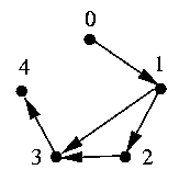
Since <0, 1> in E and <1, 3> in E,
<0, 3> is in the transitive closure of E. Since also
<3, 4> is in E, also <0, 4> is in the transitive
closure of E, i.e., node 4 is reachable from 0. In total, we have:
|
transitiveN5(E) = |
|
{<0, 1>, <0, 2>,
<0, 3>, <0, 4>, <1, 2>, <1, 3>, <1, 4>,
<2, 3>, <2, 4>}.
|
In addition, every node is reachable from itself:
|
reflexiveN5(E) = {<0, 0>, <1, 1>,
<2, 2>, <3, 3>, <4, 4>}.
|
Above definitions of closures are too inefficient for a practical algorithm
that decides the reachability of a node; a direct construction of the
reflexive closure is provided by the following result which is easy to
establish.
Proposition 132 (Reflexive Closure)
The reflexive closure of R on S is
the union of R and the identity relation on S:
|
forall S, R: R subset S x S
=> |
|
reflexiveS(R) = R union (S x S).
|
An efficient computation of the transitive closure is based on the following
operation that composes a relation R an arbitrary number of times.
Definition 131 (Exponentiation of Relations)
|
R0S :=
{<x, x>: x in S} |
|
Ri+1S :=
RiS o R.
|
RS0 is the identity relation and
RS1 is R. Consequently, e.g.
The transitive closure is then characterized by the following result which we
state without proof.
Proposition 133 (Transitive Closure)
|
forall S, R: R subset S x S
=> |
|
transitiveS(R) = union {R</sup>iS: i in N>0} |
|
|
In other words, the transitive closure of R is the union of all
members of the sequence
|
[R, R union (R o R), R union (R o R) union (R o R o R), ...]
|
that starts with R and computes each subsequent member by adding to
its predecessor the transitive consequences of
R. Since every member is contained in its successor, the transitive
closure is the "limit" of this sequence. This approach is constructive
because one can show that the sequence converges, i.e., from a certain point
on no more elements are added; the final sequence member represents the
transitive closure.
Proposition 134 (Transitive Closure)
Let R be a binary relation on S where S has n
elements. Then union_1 <= i <= n RiS is the
transitive closure of R:
|
forall S, R: R subset S x S
=> |
|
transitiveS(R) =
union_1 <= i <= n RiS |
|
where n = |S|.
|
Since the reflexive and transitive closure of the edge relation describes the
reachability relation, we thus have a constructive method of computing the
reachability relation of a graph <V, E>; we start with
the identity relation and add n times the transitive consequences of
R:
|
reachability(V, E): |
|
n = |V| |
|
R0 = {<x, x>: x in V} |
|
for (i=0; i < n; i++) |
|
Ri+1 = Ri
union (Ri o E) |
|
return Rn
|
For an actual implementation, we usually turn to the representation of the
graph as a n * n matrix M. Since in this representation
the composition of two relations resembles matrix multiplication
the computation of reachability is basically a sequence of
matrix multiplications (see this example.
Trees Trees are a special kind of graphs that are of particular
relevance in computer science: they provide a way to represent hierarchical
structures such as a family genealogy, an organizational chart, or a
file system.
Definition 132 (Tree)
A tree (Baum) is a directed graph such that there is exactly one node,
the root (Wurzel), that has indegree zero, every other node
has indegree one, and every node can be reached from the root.
|
T is tree : <=> |
|
T is directed graph /\ |
|
exists r in V:
indeg(r) = 0 /\ |
|
forall x in V-{r}: |
|
indeg(x) = 1 /\ |
|
x is reachable from r in
T |
|
where V = T0.
|
|
root(T) := (such r in V: indeg(r) = 0) where V = T0.
|
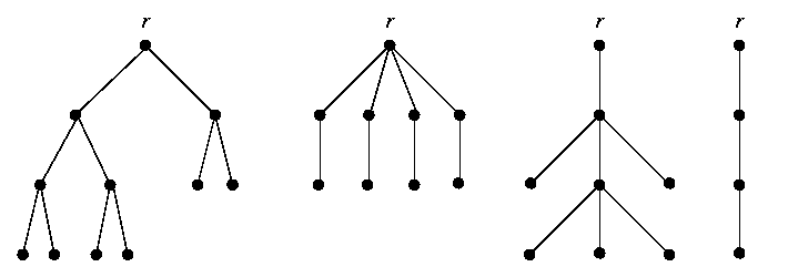
Trees are depicted with the root node at the top and all arcs directed
downwards (such that arrowheads need not be given)5.
Example
- The following diagrams depict trees with root r:
- The following directed graphs are not trees:

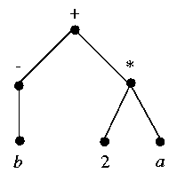
- The term -b+2a is represented by the following tree:
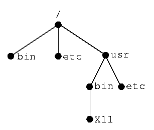
- A file system with directories
/,
/bin,
/etc,
/usr,
/usr/bin,
/usr/bin/X11,
/usr/etc
is represented by the following tree:
We state without proof the following important property of trees.
Proposition 135 (Trees and Cycles)
A tree has only cycles of length 0:
|
forall T:
T is tree => |
|
~(exists p: p is path in T /\ length(p) > 0 /\ p is cycle).
|
The following notions describe relations among tree nodes.
Definition 133 (Node Relations)
Let T be a tree. A node y is called a child (Kind) of
x if there is an edge from x to y in T:
|
y is child of x in T: <=> |
|
<x, y> in E
where E = T1.
|
x is then called the parent (Elternteil) of y:
|
parentT(y) := such x in V: <x, y> in E |
|
where V = T0, E = T1.
|
A node
x is a leaf (Blatt), if it does not have children:
|
x is leaf in T : <=> x in V /\ ~exists y: y is child of x
in T |
|
where V = T0.
|
A node x is an ancestor (Vorfahre)
of y if there is a path from x to y in T:
|
x is ancestor of y in T : <=> |
|
exists p: p is path in T /\ p is path from x to y.
|
y is then called a descendant (Nachkomme) of x:
|
y is descendant of x in T : <=> x is ancestor of y in T.
|
Please note that in a tree every node (apart from the root) has a parent and
that this parent is unique. Every node is a descendant of the root; the only
descendant of a leaf node is the node itself.
Example
In the tree
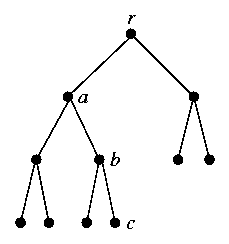
node a is the parent of b and an ancestor of leaf c.
In a tree, all paths from the root are unique.
Proposition 136 (Unique Root Paths)
Let T be a tree with root r. Then the path
from r to every node of T is unique:
|
forall T: T is tree => |
|
forall x in V: |
|
exists p: p is path in T /\ p is path from r to x
/\ |
|
forall p': (p' is path in T /\ p' is path from r to x)
=> p' = p |
|
where V = T0, r = root(T).
|
Because of this result, the following notions are uniquely defined.
Definition 134 (Level and Height)
The level (Stufe) of a node x in a tree is the length of the
path from the root of the tree to x:
|
levelT(x) := length(p) |
|
where p = such p: p is path in
T /\ p is path from root(T)
to x.
|
The height (Höhe) of a tree is the maximum level of its nodes:
|
height(T) := max
{levelT(x): x in V}
where V = T0.
|
The definition implies that the root node has level 0 and the level of a node
is one plus the level of its parent.
Example
In the tree

a has level 1, b has level 2, and c has level 3. The
height of the tree is 3.
We conclude this section by a result which relates the degrees of nodes
to the heights of trees.
Proposition 137 (Height of Binary Trees)
Let T be a tree of height h where every node has an outdegree
of at most 2. Then the number of nodes in the tree is less than
2h+1:
|
forall T: (T is tree /\ forall x in V: outdeg(x) <= 2)
=> |V| < 2h+1 |
|
where V = T0, h = height(T).
|
Proof
Let T be a tree where every node has an outdegree of at most 2. We
proceed by complete induction on the height of T.
- Assume the height is h = 0. Then
|V| = 1 < 2 = 2h+1.
- Assume the height is h > 0. Consequently the root of
T has a child that is the root of a tree of height h-1 and
possibly a second child that is the root of a tree of height less than or
equal h-1. By the induction hypothesis, we thus have
|
|V| <= 1+(2h-1)+(2h-1) = 2h+1-1 <
2h+1.
|
It is easy to generalize above result to trees whose outdegrees are bounded by
an arbutrary limit k (how?).
Author: Wolfgang Schreiner
Last Modification: October 4, 1999


