This is a brief demonstration of the integration of ProDev ProMP and the WorkShop performance tools. WorkShop must be installed for this session to work.
This sample session examines LINPACK, a standard benchmark designed to measure CPU performance in solving dense linear equations. See the SpeedShop User's Guide for a tutorial analysis of LINPACK.
This tutorial assumes you are already familiar with the basic features of the Parallel Analyzer View discussed in previous chapters. You can also consult Chapter 6, “Parallel Analyzer View Reference”, for more information.
Start by entering the following commands:
% cd /usr/demos/ProMP/linpack % make |
This updates the directory by compiling the source program linpackd.f and creating the necessary files. The performance experiment data is in the file test.linpack.cp.
After the directory has been updated, start the demo by typing:
% cvpav -e linpackd |
Note that the flag is -e, not -f as in the previous sample session. The main window of the Parallel Analyzer View opens, showing the list of loops in the program.
Click the Source button to open the loop list and the Source View. Scroll briefly through the list. Note that there are many unparallelized loops, but there is no way to know which are important. Also note that the second line in the main view shows that there is no performance experiment currently associated with the view.
Pull down Admin -> Launch Tool -> Performance Analyzer to start the Performance Analyzer.
The main window of the Performance Analyzer opens; it is empty. A small window labeled Experiment: also opens at the same time. This window is used to enter the name of an experiment. For this session, use the installed prerecorded experiment.
Click on the test.linpack.cpu directory in the directory display area, then click on the bbcounts experiment name.
The Performance Analyzer shows a busy cursor and fills its main window with the list of functions in main(). The Parallel Analyzer recognizes that the Performance Analyzer is active, and posts a busy cursor with a Loading Performance Data message. When the message goes away, performance data will have been imported by the Parallel Analyzer.
For more information about the Performance Analyzer and how it affects the user interface, see the ProDev WorkShop: Performance Analyzer User's Guide.
Once performance data has been loaded in the Parallel Analyzer View, several changes occur in the main window, as shown in Figure 5-1.
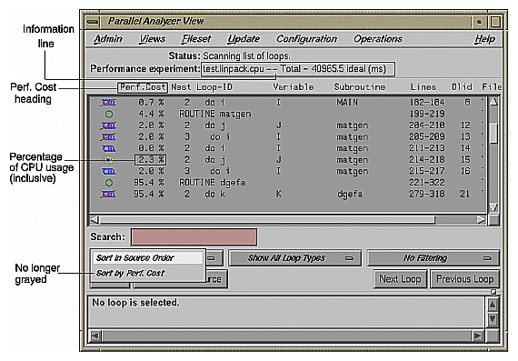
A new column, Perf. Cost, appears in the loop list next to the icon column. The values in this column are inclusive: each reflects the time spent in the loop and in any nested loops or functions called from within the loop.
The Performance experiment line, in the main view below the menu bar, now shows the name of the performance experiment and the total cost of the run in milliseconds.
The Sort by Perf.Cost option of the sort option button is now available.
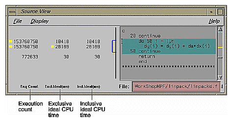
In the Source View, three columns appear to the left of the loop brackets. (These columns may take a few moments to load.) They reflect the measured performance data:
Exq Count: the number of times the line has been executed
Excl Ideal(ms): exclusive, ideal CPU time in milliseconds
Incl Ideal(ms): inclusive, ideal CPU time in milliseconds
To see the effect of the performance data on the Source View, select Olid 30, which is in subroutine daxpy(). The Source View appears as shown in Figure 5-2.
Choose the Sort by Perf.Cost sort option. Note that the third most expensive loop listed, Olid 30 of subroutine daxpy(), represents approximately 94% of the total time. (See Figure 5-3.)
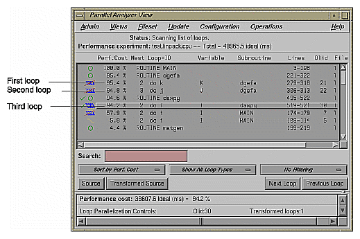
The first of the high-cost loops, Olid 21 in subroutine dgefa(), contains the second most expensive loop (Olid 22) nested inside it. This second loop calls daxpy(), which contains Olid 30--the heart of the LINPACK benchmark. Olid 30 performs the central operation of scaling a vector and adding it to another vector. It was parallelized by the compiler. Note the C$OMP PARALLEL DO directive that appears for this loop in the Transformed Source View.
The loop following daxpy() uses approximately 58% of the CPU time. This loop is the most frequent caller of dgefa() , and so of Olid 30.
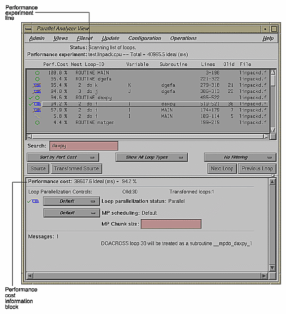
Double-click Olid 30. Note that the loop information display contains a line of text listing the performance cost of the loop, both in time and as a percentage of the total time. (See Figure 5-4.)
This completes the second sample session.
Close all windows--those that belong to the Parallel Analyzer View as well as those that belong to the Performance Analyzer and the Source View--by selecting the option Admin -> Project -> Exit in the Parallel Analyzer View.
You don't need to clean up the directory, because you haven't made any changes in this session.
If you experiment and do make changes, when you are finished you can clean up the directory and remove all generated files by entering the following in your shell window:
% make clean |